In a previous post on the problem of detecting complex financial crimes, I described the following basic technology framework for financial intelligence units (FIUs) and their partner agencies and reporting entities (REs) to engage in collaborative but privacy-preserving and distributed risk modelling using confidential computing technologies.

In this post, I describe a few concrete algorithms that can be realised in that framework. These are simple but practical algorithms that will scale to large datasets and allow the financial system to achieve a meaningful uplift in our collective ability to detect crimes.
Let’s start with the basics: distributed privacy-preserving linear regression. The following diagram shows the basic setup we are working with. Through privacy-preserving data matching techniques, we assume the different reporting entities have identified their common set of customers.

Each RE holds different variables about these customers, including but not limited to their personal information, products and services being used, risk profiles, transaction patterns, etc. The FIU holds a vector 

- no organisation can see another organisation’s raw data;
- each RE holds the weight coefficients for the variables it holds, which is not visible to others; and
- prediction of a new instance requires the collaboration of all the REs.
Linear Regression using Gradient Descent
Our privacy-preserving algorithm will be based on the Gradient Descent algorithm for linear regression, which we now describe. Given training data 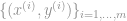


The algorithm will converge to the optimal solution since the least-squares objective function is convex. Here 
Distributed Privacy-Preserving Linear Regression
In the privacy-preserving version of the gradient descent algorithm for linear regression, we will use the Paillier cryptosystem to homomorphically encrypt data. The FIU first generates a public-private key pair and then sends the public key to the REs. The public key is used by the REs to share encrypted data and do joint computations on them. The private key is visible only to the FIU and is used by the FIU to decrypt data sent from the REs. We will also need to extend the Paillier system, which is only defined on positive integers, to floating-point numbers to support this use case, and that is explained in this post.

We next look at the learning algorithm. In the weight-update formula shown above, there are essentially two steps: a prediction step where the REs will jointly compute the predicted values 

The prediction step can be done in a privacy-preserving fashion by having the REs first locally compute the partial predictions 

The partial predictions 

In the weight update step, the FIU decrypts the predictions sent to it and then computes the gradient in the form of the difference between the predicted values (encrypted) by REs and the true values. Next, the gradient is sent back to the REs (unencrypted) and each RE then updates its own part of the weight vector independently, as shown here.

In this manner, the FIU and the REs repeatedly and jointly perform the prediction and weight update steps until the model converges. Throughout the whole computation, the FIU only sees the predicted values from the REs, from which it cannot recover the data held by the REs, and the REs only see encrypted partial predictions from each other and the gradient from the FIU, from which they cannot recover the data held by the FIU and other REs. We thus have an algorithm that can provably learn a statistical risk model across distributed datasets while preserving privacy.
A simple R implementation of the algorithm is attached at the end of the post for those who wants to experiment with it.
Beyond Linear Regression
I list a few other simple but practical algorithms for privacy-preserving distributed risk modelling here:
- The above algorithm can be easily extended to implement ridge regression by adding the
regularisation term.
- Here is a description of privacy-preserving logistic regression implemented on Data61’s N1 Analytics engine, which follows the same general algorithmic strategy above but is a bit more involved.
- Here is a previous post on Privacy Preserving Support Vector Machines: A Simple Version. The assumption there is that each party holds the exact same set of variables and data is horizontally partitioned rather than vertically partitioned like in the case for this post. Also, that post only deals with linear kernels. To handle non-linear kernels, we can work with approximations of explicitly constructed feature space; see, for example, some techniques implemented in scikit. I think it’s also possible, though I haven’t done it myself, to implement the NORMA family of online SVM algorithms to get regression, classification, and novelty-detection algorithms.
R Code
The following (unoptimised) R code shows privacy-preserving linear regression in action. The complete code can be downloaded from here.
######################################
# Set up a simple artificial dataset
######################################
n = 50
x1 = 11:(10+n)
x2 = runif(n,5,95)
x3 = rbinom(n,1,0.5)

x = data.frame(x1,x2,x3)
x = scale(x)
x = data.frame(1,x) # the intercept is handled using a column of 1's

sigma = 1.4
eps = rnorm(x1, 0, sigma) # generate noise vector

b = c(17, -2.5, 0.5,-5.2) # the real model coefficient

y = b[1] + b[2] * x[,2] + b[3] * x[,3] + b[4] * x[,4] + scale(eps) # target variable

##############################################################################
# Batch Gradient Descent algorithm, here for benchmarking and error checking
# For a refresher on the algorithm, read the first 6 pages of
# http://cs229.stanford.edu/notes/cs229-notes1.pdf
##############################################################################

lm_sgd <- function(iter, rate) {
  theta = c(0,0,0,0)
  alpha = rate
  for (iter in 1:iter) {
     adj = c(0,0,0,0)
     for (i in 1:4) {
         for (j in 1:n) {
             adj[i] = adj[i] + (sum(x[j,] * theta) - y[j]) * x[j,i]
         }
         # theta[i] = theta[i] - (alpha / n) * adj[i] # adjust as we go is faster
     }
     for (i in 1:4) theta[i] = theta[i] - (alpha / n) * adj[i]
     print(adj)
  }
  print(theta)
}

# lm_sgd(50, 0.1)

##########################################################################################
# Distributed Privacy-Preserving Gradient Descent algorithm for Linear Regression
##########################################################################################
# Basic setup:
# FIU holds the vector y of true labels
# RE1 holds the data x[,1:3]
# RE2 holds the data x[,4]
# Together, they want to learn a linear model to predict y using x but in such a way that
# - nobody sees each other's data,
# - RE1 holds the coefficients for the variables it holds, which is not visible to others
# - RE2 holds the coefficients for the variables it holds, which is not visible to others
# - Prediction of a new instance requires the collaboration of RE1 and RE2
###########################################################################################

###############################################################################################
# FIU first generates a public-private key pair using the Paillier scheme
# Public key is used by RE1 and RE2 to encrypt their data and do maths on them.
# Private key is visible only to FIU and is used by the FIU to decrypt data sent from the REs.
###########

library(homomorpheR)
source("paillier.R")  # import functions for extending Paillier to floating-point numbers
keypair = PaillierKeyPair$new(modulusBits = 1024)
pubkey = keypair$pubkey
privkey = keypair$getPrivateKey()

# Some useful constants
zero = pubkey$encrypt('0')
one = pubkey$encrypt('1')

##################################################################
# Here are the functions to setup the parties in the computation
#################

x1 = c() # these 3 vectors belong to RE1
x2 = c()
x3 = c()

re1setup = function() {
    x1 <<- encrypt(x[,1])
    x2 <<- encrypt(x[,2])
    x3 <<- encrypt(x[,3])
}

x4 = c() # this belong to RE2

re2setup = function() {
    x4 <<- encrypt(x[,4])
}

mastersetup = function() {
    re1setup()
    re2setup()
}

############
# This function computes the gradient: the difference between predicted values (encrypted) by REs and the true values
# Note the gradient is unencrypted. We could encrypt it if necessary.
#########

master_grad <- function(x) {
    xd = decrypt(x)
    xd - y
}

###########
# This is used to compute the partial predictions based on RE1's data only. The values are encrypted.
###########
re1pred <- function() {
    return (addenc(smultenc(x1, theta1),
            addenc(smultenc(x2, theta2),
            smultenc(x3, theta3))))
}

#############
# Here, RE2 takes the partial prediction of RE1 and then add its contribution to the prediction.
# The final prediction values are encrypted.
###########

re2pred <- function(z) {
    return (addenc(z, smultenc(x4, theta4)))
}

cadj = c(0,0,0,0) # a variable we want to print to keep track of progress

#############
# This is RE1's model update function and implements the gradient descent update formula.
# It takes the gradient (unencrypted) from the master and then adjust its own theta.
# The whole computation is assumed to take place within RE1 and no encryption is required.
# We can encrypt the whole thing if we want to.
###########

re1update <- function(z) {
    theta1 <<- theta1 - (alpha / n) * sum(z * x[,1])
    theta2 <<- theta2 - (alpha / n) * sum(z * x[,2])
    theta3 <<- theta3 - (alpha / n) * sum(z * x[,3])
    cadj[1] <<- sum(z * x[,1])
    cadj[2] <<- sum(z * x[,2])
    cadj[3] <<- sum(z * x[,3])
}

#############
# This is RE2's model update function and implements the gradient descent update formula.
# It takes the gradient (unencrypted) from the master and then adjust its own theta.
# The whole computation is assumed to take place within RE1 and no encryption is required.
# We can encrypt the whole thing if we want to.
###########

re2update <- function(z) {
    theta4 <<- theta4 - (alpha / n) * sum(z * x[,4])
    cadj[4] <<- sum(z * x[,4])
}

##########################################################################
# Finally, this is the privacy-preserving linear regression algorithm.
# The algorithm can be sensitive to the learning rate.
##########################################################################

pp_lm_sgd <- function(iter, rate) {

  theta1 <<- 0
  theta2 <<- 0
  theta3 <<- 0
  theta4 <<- 0
  alpha <<- rate

  mastersetup() # encrypt the data and set up communication

  for (i in 1:iter) {
      p1 = re1pred() # partial prediction
      px = re2pred(p1) # full prediction
      grad = master_grad(px) # compute gradient based on difference between true values and predicted values
      re1update(grad) # update models independently
      re2update(grad)
      print(cadj)
  }
  print(c(theta1,theta2,theta3,theta4))
}

model0 = lm_sgd(100, 0.1)
model1 = pp_lm_sgd(100, 0.1)

One thought on “Practical Algorithms for Distributed Privacy-Preserving Risk Modelling”