Mental Models 4 Life

I have just received the excellent news that Apache MADlib, a big data machine learning library for which I was a committer until recently, has graduated to become a top-level Apache project.

The basic idea behind MADlib is actually quite interesting and deserves to be more widely known. Massively Parallel Processing (MPP) databases like Greenplum have been around for a while and they provide us with a convenient way to process terabyte-scale data using mostly standard SQL. The insight behind the development of MADlib is simply this: if only we can write machine-learning algorithms in SQL (that’s the mental leap required), then running those SQL code on MPP databases will allow us to learn machine-learning models on terabyte-scale data, something that’s impossible to do on traditional memory-constrained systems like R, S, SPSS, etc.

I can hear you, the reader, questioning the wisdom of trying to write machine-learning algorithms in SQL. It’s not completely obvious how that can be done, but there are a few design patterns that can help us. Let’s look at one such pattern to get some intuition, starting with an example machine learning problem.

Suppose you want to do automated face recognition. You have a dataset of faces associated with a known entity and you want to learn a statistical model that will allow you to go searching for possible matches in the rest of your database of images.

One idea is to represent each image as a point in some n-dimensional space. And if images associated with different people are nicely separated, then we can use a hyperplane to distinguish between people.

This is obviously a simplistic view, but there are several quite sophisticated machine learning algorithms that are built upon that basic intuition. One very successful one is the support vector machines (SVMs).

Let’s take crash course on SVMs, starting with a quick formulation of the class of models. We start with a kernel function, that given two data points, gives a measure of the ‘similarity’ between the two points. Associated with such a kernel function is a space H of functions called the reproducing kernel Hilbert space, where each function in H is a weighted sum of kernel functions.

In the case when k(.,.) is the inner product, H is the set of all hyperplanes.

The machine learning problem is to search for the model that best fits our data in the set H of possible models. A model for “being JT” may look like this:

Recall that k(x,y) measures the similarity of x and y. So the model above simply measures how well a face matches each of the distinctive faces listed. Some of the distinctive faces corresponds to positive correlation with being JT, others give a negative correlation.

To classify a new face using the model, we just plug in the new face. If the result is a positive number, it’s JT. Otherwise, no.

We next formulate the SVM optimisation problem. Given data S, the SVM optimisation problem is to find a model f in H that minimises the error function

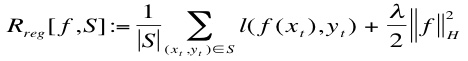where the first term captures how well the model f fits the training data, and the second term is a way of measuring the complexity of f.

There are many ways to solve the optimisation problem, but most of them are not really scalable. One technique that is scalable is the idea of online learning. The idea is simple: when you have a large amount of data such that it’s impossible to load all of them into memory at the same time, what you can do is process the data one at a time using an incrementally maintained model, where we adjust the model every time we make a prediction error.

There’s a surprisingly simple way to implement such online algorithms in SQL using user-defined aggregate functions, and that’s our first design pattern for implementing machine-learning algorithms in SQL.

Let’s see how this will work in practice for SVMs. If we use stochastic gradient descent to solve the SVM optimisation problem, we get this algorithm (see Kivinen et al 2003 for the mathematical derivation):

is the margin. We have is positive if we make a correct prediction with high confidence, in which case we do nothing. But if we make a prediction error or make a right prediction but with low confidence, then we adjust the model by discounting it and then adding a new term corresponding to the example we have just mis-predicted. (In the case of our earlier face-recognition problem, the faces that end up in the model are the ones that we misclassified along the way, which shows that those are the most important or distinctive faces to remember!)

Now let’s look at how we can implement this algorithm in SQL, using Greenplum as an example MPP database.

It couldn’t be simpler, really. We first define a user-defined function (UDF) that implements the iterative step of the online SVM algorithm.

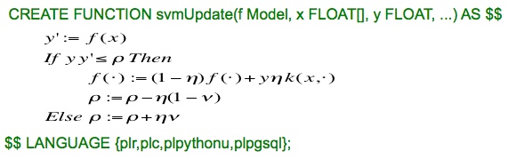
This can be done in any number of languages, including R, Python, or PL/pgSQL.

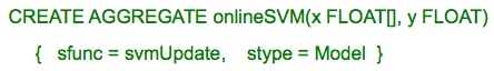
We then create a new aggregate function, call it onlineSVM, and declare that the state of that aggregate function is an SVM model, and that the state transition function is the svmUpdate UDF we’ve just defined.

Now we are in a position to learn SVM models from large datasets, and this is the SQL code to do it.

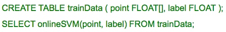
Here, we have Ÿessentially one simple algorithm (~20 lines of code) to do classification, regression, and novelty detection on massive data sets unconstrained by main memory. Isn’t that just a beauty?

That’s the first design pattern for implementing machine-learning algorithms in SQL. We’ll look at one more pattern: parallel ensemble learning. The basic idea is to break a large table into independently and identically distributed subsets of data sitting on each node in a cluster, learn a model on each subset in parallel, and then combine the models appropriate at the end. Examples of such algorithms include random forests and ensembles of SVMs.

We will again use SVMs to illustrate the design pattern on Greenplum. This time we want to learn an ensemble of SVMs, not just one. We first create a table to store the training data, and use distributed randomly to make sure each subset has the same distribution as the whole dataset.

Ensemble SVM learning can then be done just like before, but with the addition of a GROUP By gp_segment_id clause.

Each row in a Greenplum table has a field called gp_segment_id which tells us where the row resides in the underlying database. The group by statement tells the system to do a separate onlineSVM() aggregate on the subset of data residing on each node. The above SQL example also gives us some hints on the ways SQL can be used to convey parallel processes that can be recognised and executed by the planner.

There are many more design patterns that are used in MADlib to implement machine learning algorithms in SQL. I hope the above illustration demystifies some of the magic in MADlib code.