Mental Models 4 Life

While doing a project involving survival analysis a while back, I learned a useful technique for reducing survival analysis to binary regression. The following discussion is adapted from Chapter 7 of Survival Analysis by David G. Kleinbaum.

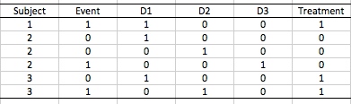
To illustrate how the technique works, consider a small data set with three subjects. Subjects 1 and 3 are administered a certain treatment for an “event” while Subject 2 is the control. From subsequent follow-ups, we learned that Subject 1 got the event in the first interval, Subject 2 got the event in the third interval, and Subject 3 got the event in the second interval.

To turn the data into a form suitable for binary regression, we introduce three dummy variables D1, D2, D3 which are coded 1 if we are in the corresponding interval and 0 otherwise. This yields the following table:

A logistic regression model can then be formulated as

,

where Pr(Event = 1) is the probability of the event under study for a given interval conditioned on survival of previous intervals.

The dummy variables play a similar role to that of the intercept in a standard regression model: it provides a baseline outcome, one for each interval, in the case where all other variables are zero.

This is how we interpret the coefficients: is the log odds of the event occurring in the first interval among the control group; is the log odds of the event occurring in the second interval conditioned on survival of the first interval among the control group; is the log odds of the event occurring in the third interval conditioned on survival of the first two intervals among the control group; and is the log odds ratio for the Treatment variable.

Why is this technique useful?

1. While logistic regression is now a standard feature on big data platforms, some scalable machine learning libraries do not yet support survival analysis models like hazards models. The technique described here is a way around such constraints.
2. Technical folks who are not otherwise familiar with survival analysis seems to have an easier time understanding this alternative formulation of survival analysis compared to the more standard hazards models.
3. The alternative formulation easily supports time-dependent variables which are not easy to handle in standard hazards models.
4. The alternative formulation also allows us to move beyond linear models for survival analysis. Any machine-learning algorithm that deals with binary regression can now be considered.