Have you ever wondered why the natural exponential function shows up so frequently in mathematical inequalities?
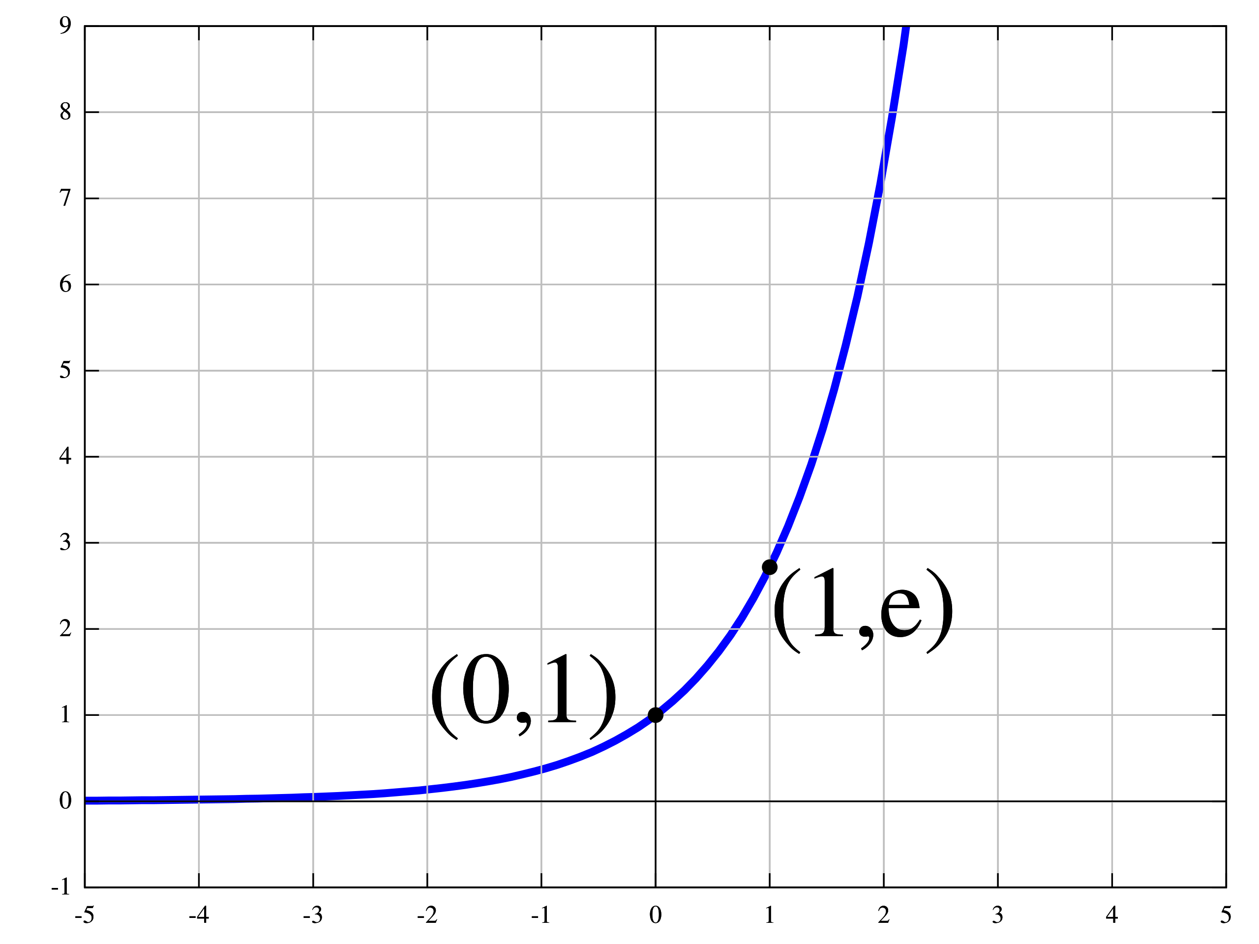
Here’s a graph of the natural exponential function.
The constant e has a special place in mathematics, which is beautifully chronicled in Eli Maor’s book [M94]. The definition of e that is most useful and intuitive for our purpose is this: , which can be understood as the rate of growth if we compound a quantity at 100% growth rate over a fixed time period [a,b] by dividing the period into n smaller and smaller time intervals. (See this short article if you want to see how things change in an interesting way with different growth rates and time periods.) From the above definition of e, one can derive arguably the most important property of e, which is that . (Here is an intuitive proof from KhanAcademy.) In other words, the growth rate at an any point x is so, as one can see in the graph above, as x increases, the growth rate increases at an exponential rate, giving us the magic of compounding. From the perspective of proving mathematical inequalities, especially when we want to put an upper bound on the probability of some “bad event” happening, it is the left-end tail of the natural exponential graph that is interesting, in that as x decreases, the “growth” rate quickly turns negative into an exponentially increasing rate of decline!
The other key property of the natural exponential function is that it is convex, which means one can use Taylor’s Theorem to find a lower bound to the function at a specific point y using a polynomial expressible in y and derivatives of , which is usually easy to manipulate given the derivative of the natural exponential function is itself. The convexity property also allows us to use Jensen’s Inequality to provide bounds on linear combinations of the exponential function, and that is especially useful for proving inequalities on the expectation of random variables expressible using the exponential function. In fact, Hoeffding’s Lemma, which states that for a random variable X that takes value in a bounded range [a,b] and any real number s,
has an elementary proof that only uses the convexity property and Taylor expansion. (See, for example, Appendix A.1.1 in [CL06].) Using Hoeffding’s Lemma, the incredibly useful Hoeffding’s Inequality for the convergence of the sum of multiple i.i.d bounded random variables can be obtained as a special case of Chernoff Bound, which can itself be obtained from the elementary Markov’s Inequality, which states that for any non-negative random variable X and non-negative epsilon, by substituting X with the random variable for a positive lambda.
Indeed, motivated by Hoeffding’s Lemma and the Gaussian distribution, we can define the following important class of random variables that have “nice” tail probabilities that drop off quickly: A random variable X is sub-Gaussian if, for any real number s,
for a given positive constant called variance proxy. The nice thing about sub-Gaussian random variables is that they satisfy Chernoff’s Bound and, in particular, they have a moment generating function that is uniformly bounded above by the moment generating function of a Gaussian random variable, which means the tail probability drops off at least as quickly as that of the Gaussian distribution. Obviously, Gaussian random variables are sub-Gaussian. Any bounded random variable is sub-Gaussian with variance proxy by Hoeffding’s Lemma. Also, any linear sum of sub-Gaussian variables is itself a sub-Gaussian variable, which allows us to prove bounds like Hoeffding’s Inequality for i.i.d data that underlie much of the theory of supervised machine learning. In fact, sub-Gaussian random variables play a major role in the phenomenon of concentration of random variables, which can be stated informally as follows:
If are independent (or weakly dependent) random variables, then the random variable is “close” to its mean provided that the value of is not too sensitive to changes in only one of the variables at a time.
Indeed, the famous McDiarmid’s Inequality, which states that for independent random variables and arbitrary function f,
where can be proved by showing that each incremental change is bounded and therefore sub-Gaussian by Hoeffing’s Lemma, and the sum is sub-Gaussian. (See, for example, [BLM13] for a detailed treatment.)
There remains two other things to quickly mention. We stated above that the moment generating function of a sub-Gaussian random variable is upper-bounded uniformly by the moment generating function of a Gaussian distribution. It’s worth recalling that the moment generating function of a random variable X is defined by , which is so-named because it generates all the moments of X through the Taylor series for to yield
.
This ability for us to lay out all the moments of a random variable is useful in many problems.
Finally, the natural exponential function also satisfy a couple of elementary inequalities like for all x, and for all . These simple inequalities sometimes give bounds that are only worse off by a small constant compared to Hoeffding’s Lemma so it’s worth starting with those to see where you get to.
References
[M94] Eli Maor, e: The Story of a Number, PUP, 1994.
[CL06] Nicolo Cesa-Bianchi and Gabor Lugosi, Prediction, Learning and Games, CUP, 2006.
[BLM13] Stephane Boucheron, Gabor Lugosi, Pascal Massart, Concentration Inequalities: A Nonasymptotic Theory of Independence, OUP, 2013.


![\ln \mathbb{E}[ e^{sX} ] \leq s \mathbb{E}[X] + \frac{ s^2 (b-a)^2 }{8}](https://s0.wp.com/latex.php?latex=%5Cln+%5Cmathbb%7BE%7D%5B+e%5E%7BsX%7D+%5D+%5Cleq+s+%5Cmathbb%7BE%7D%5BX%5D+%2B+%5Cfrac%7B+s%5E2+%28b-a%29%5E2+%7D%7B8%7D&bg=ffffff&fg=888888&s=0&c=20201002)
![Pr( X \geq \epsilon ) \leq \mathbb{E}[X] / \epsilon](https://s0.wp.com/latex.php?latex=Pr%28+X+%5Cgeq+%5Cepsilon+%29+%5Cleq+%5Cmathbb%7BE%7D%5BX%5D+%2F+%5Cepsilon&bg=ffffff&fg=888888&s=0&c=20201002)

![\mathbb{E} e^{s (X - \mathbb{E}[X])} \leq e^{\sigma^2 s^2 / 2}](https://s0.wp.com/latex.php?latex=%5Cmathbb%7BE%7D+e%5E%7Bs+%28X+-+%5Cmathbb%7BE%7D%5BX%5D%29%7D+%5Cleq+e%5E%7B%5Csigma%5E2+s%5E2+%2F+2%7D&bg=ffffff&fg=888888&s=0&c=20201002)


![\mathbb{E}[f(X_1,\ldots,X_n)]](https://s0.wp.com/latex.php?latex=%5Cmathbb%7BE%7D%5Bf%28X_1%2C%5Cldots%2CX_n%29%5D&bg=ffffff&fg=888888&s=0&c=20201002)


![Pr(f(X_1,\ldots,X_n) - \mathbb{E}[f(X_1, \ldots, X_n)] \geq \epsilon) \leq e^{-2\epsilon^2 / \sum_{i=1}^n || \delta_i f ||_{\infty}^2}](https://s0.wp.com/latex.php?latex=Pr%28f%28X_1%2C%5Cldots%2CX_n%29+-+%5Cmathbb%7BE%7D%5Bf%28X_1%2C+%5Cldots%2C+X_n%29%5D+%5Cgeq+%5Cepsilon%29+%5Cleq+e%5E%7B-2%5Cepsilon%5E2+%2F+%5Csum_%7Bi%3D1%7D%5En+%7C%7C+%5Cdelta_i+f+%7C%7C_%7B%5Cinfty%7D%5E2%7D+&bg=ffffff&fg=888888&s=0&c=20201002)

![\Delta_i = \mathbb{E}[f(X_1,\ldots,X_n) \,|\, X_1,\ldots, X_i] - \mathbb{E}(f(X_1,\ldots,X_n) \,|\, X_1, \ldots, X_{i-1}]](https://s0.wp.com/latex.php?latex=%5CDelta_i+%3D+%5Cmathbb%7BE%7D%5Bf%28X_1%2C%5Cldots%2CX_n%29+%5C%2C%7C%5C%2C+X_1%2C%5Cldots%2C+X_i%5D+-+%5Cmathbb%7BE%7D%28f%28X_1%2C%5Cldots%2CX_n%29+%5C%2C%7C%5C%2C+X_1%2C+%5Cldots%2C+X_%7Bi-1%7D%5D&bg=ffffff&fg=888888&s=0&c=20201002)
![\sum_{i=1}^n \Delta_i = f(X_1,\ldots,X_n) - \mathbb{E}[f(X_1,\ldots,X_n)]](https://s0.wp.com/latex.php?latex=%5Csum_%7Bi%3D1%7D%5En+%5CDelta_i+%3D+f%28X_1%2C%5Cldots%2CX_n%29+-+%5Cmathbb%7BE%7D%5Bf%28X_1%2C%5Cldots%2CX_n%29%5D&bg=ffffff&fg=888888&s=0&c=20201002)
![M_X(s) = \mathbb{E}[ e^{sX} ]](https://s0.wp.com/latex.php?latex=M_X%28s%29+%3D+%5Cmathbb%7BE%7D%5B+e%5E%7BsX%7D+%5D&bg=ffffff&fg=888888&s=0&c=20201002)

![M_X(s) = \mathbb{E}[ e^{sX} ] = \sum_{k=0}^{\infty} \mathbb{E}[X^k] \frac{s^k}{k!}](https://s0.wp.com/latex.php?latex=M_X%28s%29+%3D+%5Cmathbb%7BE%7D%5B+e%5E%7BsX%7D+%5D+%3D+%5Csum_%7Bk%3D0%7D%5E%7B%5Cinfty%7D+%5Cmathbb%7BE%7D%5BX%5Ek%5D+%5Cfrac%7Bs%5Ek%7D%7Bk%21%7D&bg=ffffff&fg=888888&s=0&c=20201002)


